Ragged Hierarchy Navigation

Ragged Hierarchies are a common BI reporting structure in which the hierarchy contains a variable number of levels.  Examples are an organization hierarchy, or a financial chart of accounts.  Ragged hierarchies are cumbersome to navigate using standard SQL.  But there are ways to simplify the navigation without compromising performance. 

It is useful to employ a “tree” metaphor to visualize the modeling challenges of dimensional hierarchies.  A “tree” is a collection of reporting hierarchies such as may exist in a product dimension or an organization dimension.  A tree consists of “branches” that represent the levels of a hierarchy.  Each branch contains one or more “nodes”.  A node can be a “leaf” or another branch.  A leaf is the most granular node of a hierarchy, and is referred to as a “leaf node”.  Each leaf node contains the values of the various attributes of the dimension.  The set of all nodes emanating from a given branch node is referred to as a “sub-tree”.  A single “hierarchy” is the set of connected nodes between a given node and the trunk. The “trunk” represents the collection of all hierarchies in the dimensional tree. 
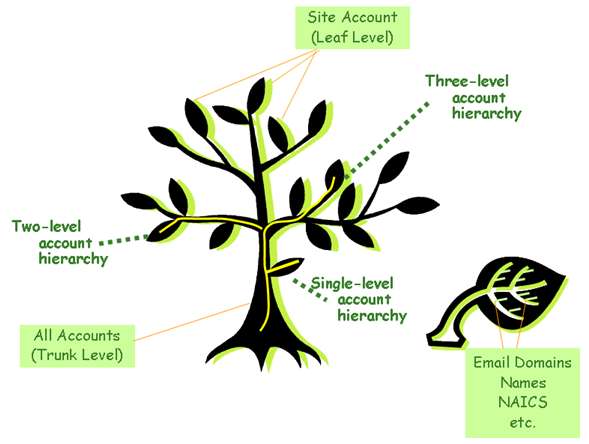
 

Hierarchy Navigation Tree

A “ragged hierarchy” exists when the number of levels varies between hierarchies.  Figure 1 depicts an Account dimension with ragged hierarchies.  Three hierarchies are highlighted including a single, double, and triple level hierarchy.

Recursive Hierarchies

Hierarchies are often modeled using “parent keys” in the dimension table.  A dimension exhibits recursive hierarchies when there can be two or more levels of levels of parent-child relationships in the same table.  Dynamically navigating recursive hierarchies with a BI tool like Cognos or Business Objects is expensive. Each level requires a self-join. There are two basic types of dimension recursive hierarchies. 

Fixed Recursive Hierarchies

If the number of levels in the hierarchy is fixed, then the dimension table contains fixed recursive hierarchies.  An example is a standard product or merchandise hierarchies (e.g. family > class > commodity > category > item).  Because the number of levels is known, the dimensions can be modeled with parent key column for each level of the hierarchy.  However, this does not necessarily eliminate the need for recursive joins at query time.

Dynamic Recursive Hierarchies

If the number of levels in the hierarchy is indeterminate, then you have a ragged recursive hierarchy.  Project and organization hierarchies are typically ragged.  For example, a project may have one or more sub-projects, each of which could have its own sub-projects. 

Left outer joins are required to navigate each level of a recursive hierarchy.  If the dimensions are large and there are many levels in the hierarchy, performance could become an issue.  It is not always possible to optimize recursive joins because the parent-key column functions as both a parent and a child. You cannot co-locate the parent and child rows on the same Netezza SPU.  In databases like Oracle that use indexes,  separately indexing the primary key and the parent key may offer some performance relief, but performance will still degrade as the number of levels (and therefore joins) increases. 

Hierarchy Navigation Tables

A ragged hierarchy is simplified by creating a hierarchy navigation table in the database.  Navigation tables can be directly queried by the BI tool without expensive recursive joins.  Navigation tables can be optimized because the normal table joins are predictable, few in number, can be inner joined, and can be co-located with the main dimension table.  There are two basic types of hierarchy navigation tables.

Vertical Navigation Tables

Vertical navigation tables contain a row for every level of every hierarchy.  Thus, the leaf node is repeated for each level represented in its hierarchy.  If a user wanted to roll-up costs to a mid-level node in the project hierarchy, they would simply select that node, and the navigation table would make a single join to the fact table, regardless of the number of levels in the hierarchy.  Vertical navigation tables are useful when the user does not know the level the hierarchy they are querying.

Horizontal Navigation Tables

Horizontal (i.e., flattened) navigation table contain one row per hierarchy.  The levels of the hierarchy are represented as columns.  Thus, a horizontal navigation table will have fewer rows than a vertical navigation table for the same dimension. Horizontal navigation tables are useful when the user is selecting a specific level, or needs to display the parent path levels in a query or report.

Ragged Hierarchy Special Requirements

There can be variations in requirements within the general theme of ragged hierarchies.  As usual, the devil is in the details.  Specific modeling techniques to achieve optimum performance depend on the customer’s unique requirements.  Examples of special hierarchy scenarios are described below.

Multiple Parent Nodes

This scenario breaks the strict hierarchical relationship of the dimension.  A node can have 2 or more parents.  For example, a project can be a member of two different “programs” at the same time.  This requirement presents unique roll-up challenges.

Facts Attached to Multiple Levels

This scenario often exists in organizational hierarchies.  Each organization has a budget and is responsible for the budgets of the organizations within its span of control. For example, Division A is responsible for the budges of Departments 1, 2 and 3.  Department 1 is responsible for Units 1.a and 1.b.  Thus, expense roll-up queries might include costs of the Division A sub-tree including, or excluding, the Division A’s own expenses.

Versioned Hierarchies

Versioned hierarchies exist when the relationships of a hierarchy changes over time, and there is a requirement to report based on the hierarchy structure in effect as-of a point in time.  For example, customer ownership relationships may change over time as a result of mergers and acquisitions.

Approach to Optimizing Ragged Hierarchies

Optimizing Ragged Hierarchies is a four-step processes as depicted in Figure 2.

Ragged Hierarchy Optimization Approach
  1. Requirements Analysis – The first step to optimizing ragged hierarchies is to identify the business requirements.  What is the general model and what are the special requirements?   The requirements analysis will narrow down the optimization options.
  2. Business Rule Modeling– The second step is to allocate business rule processing between the BI query tool, the database structures, and the ETL application.  The choices will depend on the query use cases, the capabilities of the BI tool, and service level agreements (SLAs) related to query response times and available ETL batch window times.
  3. Data Modeling – The third step involves modeling the dimensions, navigation tables, and the database tables and views required to support the loading and navigation of ragged hierarchies.
  4. Physical Optimization – The fourth step is to optimize the physical database structures based on performance tests.  The results will depend on a variety of factors including data volumes, hierarchy versioning requirements, the distribution of data, the frequency of updating the hierarchies, and the user query profiles.  Physical optimization may lead to adjustments in steps 2 and 3.

***********

In summary, ragged hierarchies are a fact of life in the ragged real world.  Hopefully the techniques in this post will help you smooth things over with your users 🙂   I would love to hear your feedback on these and other approaches for handling ragged hierarchies.
Business Analytics Modeling Demonstration Project

Business analytics are the distillation of “big data” that is actually used to make decisions.  Surprisingly, business analytics are rarely included in the data models used to build the EDW.  More often, BI designers model analytics in the BI tool metadata, assuming that the EDW data model and physical structure will support those analytics.  Surprises occur at this point!  This project suggests best practices and tools for integrating business analytics into the EDW data modeling process to create better BI solutions.

What is a Business Analytics Data Model?

BI solutions typically involve many thousands of data objects.  BI dimensional data modeling is often tasked to capture all “potentially useful” source elements for the target subject area.  This largely source-driven approach can lead to a “boil the ocean” effort that delays the deployment of useful BI reporting.  To enable a more direct path to BI results, business analytic objects are integrated with the BI dimensional model.  The process is a convergence of source/target-driven and analytics-driven modeling.

A Business Analytic Data Model is an enriched form of the BI dimensional data model that includes analytic data objects.  Analytic data objects directly influence manual or mechanized decision making, are predictive as well as historical in nature, and can be derived from structured and non-structured data.

Business analytics are the lynch-pins that unite business requirements analysis with data modeling.  Data requirements emerge by decomposing the business analytics.  Modeling from business analytics to the required data reveals gaps or structural problems in the data model that might be missed by traditional source-to-target BI dimensional data modeling.  Each approach compliments the other in getting to the best solution in the shortest time.

What are the Goals of a Business Analytics Data Model?

Business analytics modeling can help solve three major BI/EDW challenges:

    1. Aligning business and IT stakeholders in the process of developing of BI/EDW solutions
    2. Ensuring that the EDW data model will support the business reporting requirements
    3. Establishing a framework for overall business performance management

On the surface, these challenges read like general requirements that would apply to any BI/EDW initiative. But why are they so incredibly difficult to achive?  And how can a business analytics model help?  Let’s address those questions one at a time.

Aligning Business and IT Stakeholders

IT and business stakeholders want the same thing in the end — a succesful BI solution that benefits the organziation and all involved.  But they approach the journey from different perspectives.

IT-Business Alignment

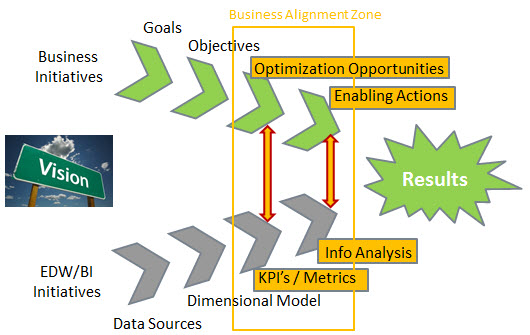
There is a critical point where the business and IT journeys converge, and that is when the business analytics are formulated.

BUSINESS VIEW: Business analytics measure the optimization opportunity — How well are we doing?  How big is the prize?  Analytics suggest or trigger enabling actions to achive the opportunity.

IT VIEW:  Business analytics are the nucleus of a mini-data model that collectively stretch into all corners of the dimensional model, and back to the data sources.

If we can get the IT and business collaboration right during this critical stage, the probablity of a successful BI/EDW result will be improved.  Future posts will present some business analytics modeling methods, and pitfalls to avoid, gleaned from many BI projects undertaken by Brightlight and yours truly.

Ensuring that the EDW data model SUPPORTS business analytics reporting

<in process>

Establishing a framework for business performance management

<in process>

************

I would like your insights on business analytics modeling challenges you have encountered at your companies.  Please use the comment form at the end of each post.  I will respond and try to incorporate your ideas into the demonstration project.

Flexible Hierarchies Demonstration Project

Business hierarchies are the “crown jewels” of an analytic-driven organization.  They encode the analytic framework for marketing, product and sales management, and competitive benchmarking.  This project will walk you through the steps to create a high-performing EDW model for dynamic, flexible business hierarchies.  The project will provide technical artifacts for a Netezza DW appliance solution, but the modeling concepts are applicable to other EDW platforms.  I will post on this site progress of this project journey, and invite your suggestions and stories from your own experiences.  You can reply using the commenting dialog at the end of each post.

In this project I will layout a modeling approach and a prototype for hierarchies that work the way you want, and they way Chelsea in finance wants, and Joe in marketing wants, and your merchandising director and suppliers want.  The result is a compendium of approaches I have used at various clients in several industries over the last six years, born out of lot of listening and technical experimentation, and tempered with published research from DW gurus like Ralph Kimball and Joe Celko.  I’m certain to have violated some rules along the way, but my view is that things that actually get used leave a trace of broken rules in pursuit of the greater good.

First, the requirements.  Below is a list of “We needs” that come up time again when discussing hierarchy requirements with business folks:

    • We need to report the same sales data by different roll-up hierarchies
    • We need hierarchies that can report summary results consistently across business units.
    • We need hierarchies that support a variable number of levels (aka, “ragged hierarchies”)
    • We need to link related hierarchies–for example, sales organization hierarchy linked to product hierarchy
    • We need to track hierarchy changes so we can report based on the hierarchy structure today, or at any historical date.
    • We need to evaluate the impact of planned hierarchy changes simultaneously with current reporting.
    • We need to integrate external product or customer data with our internal hierarchies.
    • We need to update hierarchies with known changes in advance of the delayed feeds from external data suppliers.
    • We need to navigate the hierarchy in various ways depending on the business question.
    • We need to dynamically aggregate facts by hierarchy level or node.
    • We need to track multiple occurances of attributes such as addresses, industry codes, etc.
    • We need to handle hierarchy nodes with more than one parent (e.g, a store served by two distribution centers).
    • We don’t want to update the fact table(s) when a hierarchy changes.
    • We don’t want to rely on “meaningful identifiers” that become outdated and lead to confusion.
    • We need to build in health checks alert us to inconsistencies in the hierarchies that could distort reporting.
    • We need a standardized approach to building hierarchies that is repeatable and easy to maintain.
    • Importantly, we need to make the user interface simple and intuitive.

Whew!  That is a tall order.  When hierarchies are inflexible or difficult to change, it is nearly impossible to address more than a few these needs.  Many organizations learn to live with inflexible hierarchies.  We must change that paradigm.  The value of business nimbleness that flexible hierarchies enable will far exceed the the investment to create them.

***********

Look for upcoming posts describing a conceptual architecture for flexible hierarchies, and demonstrating an industry use case.  In the meantime, please send me hierarchy challenges you have seen in your own organizations, and I’ll reply and/or incorporate them into the demo.  Use the commenting box below.


Cohort Analysis — understanding your customers

Dimensional BI analysis is great stuff for understanding the business, but what really makes your customer’s tick? BI techniques such as survey analysis, market basket analysis, and clickstream analysis help illuminate this universal question. But BI queries typically tells us about the “average customer” who never exists.  How many households do you know with exactly 2.6 people?   
 
Cohort Analysis comes at the customer question from a different direction. The idea is to choose specific customers first, and then dimensionally analyze their actions, and the reactions of related parties. This approach eliminates error resulting from changes in the underlying customer mix over time. In effect, the data warehouse becomes a massive pool of longitudinal study participants whom you don’t have to pay, and can be studied in seconds rather than years.

Stepwise Analysis 

Cohort Analsis is a three step process:

  1. The “design step” frames the question or hypothesis to investigate. For example,—do free breakfast upgrades measurably improve business traveler retention for a hotel chain? If there is a good correlation, then a check-in rule might be instituted to upgrade certain types of guests when room availability hits certain thresholds.
  2. The “cohort step” selects the customers to study,typically a control group and one or more target groups.  For example, “select from the EDW a list of business travelers based in the north-east market with at least one stay per quarter over the preceding four quarters”.  From this pool frequent travelers, subset a control group that did not receive the upgrades in the first quarter, and a target group that did.
  3. The “study step” compares the control and target cohorts over some time range and dimensional grouping criteria.  Any metrics or target groupings can be used in the comparisons.  Example metrics are number of stays, length of stays, revenue, non-room charges, etc.  Example dimensional groupings are weekend versus non-weekend guests, guests that had meal charges versus those that did not, etc.

Power to the People 

Ad-hoc cohort analysis requires raw horsepower for dynamic joins at the customer key level. Without the power afforded by an EDW, development staff may be needed to set up temporary database structures and batch processing–not good.  We want the business analyst to be in full control–commanding rapid study cycles in the iterative question?answer?next question approach.  For performance reasons, cohort analysis processing should take place mostly on the EDW server, not the reporting tool platform.  In addition, certain aggregate tables and views may be required in the back-end EDW. 

Cohort Analysis Workbench

A Cohort Analysis Workbench enables the analyst to save cohort stage result sets for later use as study filters.  The workbench also manages a folder-based library of cohorts and studies for comparative analysis. High-end BI tools like MicroStrategy are well suited for creating such a workbench.  MicroStrategy can publish intermediate results to SQL tables, join reports using multi-pass SQL, and manage a library of studies with appropriate security. 

A Collaborative Approach 

This is not entirely an out-of-the box solution.  The workbench should be explicitly designed and tested with a portfolio of templates and key metrics.  Fortunately, high-end BI tools and MPP EDW servers make building a cohort analysis workbench relatively quick task.  But business analyst and the BI analyst must collaborate closely to get the job done. The active ingredient is the brain of the lead business analyst.  His or her vision, sponsorship, enthusiasm and direct participation will assure success. 

* * * * *

Do you have opportunities for cohort analysis in your organization?  Comment back to this post with your objectives and challenges.  Let’s get some dialog going around this very powerful method for understanding your customers.

The EDW and Customer Matching

The Customer Match Challenge 

Matching and linking customer records is at the heart of Customer Data Integration (CDI).  The goal is to achieve a “360 degree view” of your customer, including past and present relationships.  There are so many challenges to this task that it can seem overwhelming.  The matching algorithms themselves are computationally intensive, consuming valuable clock time, not to mention computing resources.  Customers exist in a web of relationships with companies, groups, and other individuals.  Even if a company holds data on the various entities of the customer relationship web, that data is often scattered across systems.  Connecting the dots is a singular challenge.

Ultimately, customer matching is a learning process.  The more you know about your customer, the better able you are (or should be) to match his or her transactions.  In the real world, we usually don’t have the luxury of “retroactively” applying lessons learned.  With CDI, we are given a chance to correct prior matching mistakes.  But this opportunity is a supreme challenge architecturally.  Even if the technical challenges can be met, the business value of accurate customer matching is realized only when the information is delivered to the right place at the right time.  The CDI matching solution demands the best integration of technologies and business processes that we can possibly muster.  

While there are no silver bullets to the customer matching challenge, the EDW can fulfill a pivotal role.  This post is intended to generate discussion and ultimately lead to some principles for positioning the EDW as the hub of the CDI solution.

The Architectural Problem

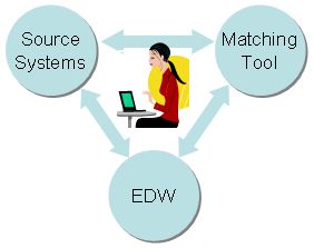
At the risk of oversimplification, let’s reduce the customer matching architectural problem to three main players—the source systems, the EDW, and the matching tool.  The source systems capture customer business transactions.  The EDW holds integrated customer profile information and granular business transactions.  The matching tool identifies distinct customers, and matches business transactions to customers based on complex matching rules.  The nature of the linkages between these three players are many and varied.  Depending on requirements, the linkages may need to be traversed in batch, real time, or near real time windows.
 

Fig. 1:  Customer Matching Players
Fig. 1: Customer Matching Linkages

Source to EDW – This is the normal ETL flow in which matched customer transactions and business profile updates are submitted to the data warehouse.  The question is—where in the data flow are the transactions matched? 

EDW to Source– This data flow direction does not exist in the traditional data warehouse model.  But with CDI, it may be necessary to synchronize source systems with the latest customer identities in the EDW.

Source to Matching Tool – Transactions are submitted to the matching tool for assignment of a customer match identifier .  The match identifier may represent a group of one or more candidate customer identifiers (i.e., “suspects”).  If the match score is sufficiently high, the transactions are assigned a distinct “golden” customer identifier.

Matching Tool to Source – The matching tool actively participates in assigning customer identifiers to the source transactions.  This could be a batch file of matched transactions, or a message of match candidates for a single customer interaction.

Matching Tool to EDW – In addition to assigning customer identifiers to source transactions, the matching tool is responsible for coming up with a distinct “golden” identity of each customer.   Customer identity information must then be stored in the EDW as a conformed and universally accessible customer dimension.

EDW to Matching Tool – The EDW is the keeper of intelligence about customers.  It is also the place where vast amounts of detail data are integrated, grouped, linked, and enriched.  Thus, the EDW is a logical source of data for the matching tool.  The EDW can relieve the matching tool of the data management responsibility so that it can concentrate fully on the matching tasks.

Note that successful customer matching requires a dose of human intervention at key points.  The need for human participation contributes to decisions about which processes should take place in “interaction windows” versus “batch windows”.  An interaction window is the time frame during which a business transaction involving people is consummated.  A batch windowis an arbitrary time frame during which data is processed after the fact, without influencing the originating business transactions.

Designing customer matching linkages that balance business requirements with technical feasibility is a key architectural challenge for a successful CDI implementation.    Pragmatism is your good counsel in this endeavor. 

How Can the EDW Help?

The Enterprise Data Warehouse can and should play a central role in the CDI architecture.  The main idea is that it is much easier to synchronize data around a common customer definition when the data to be synchronized exists in one place.  Setting aside for the moment the question of whether the EDW should exist as a source of record for customer data (i.e., a CDI “transactional hub”), let’s just say that maintaining a 360 view of the customer in an EDW is more natural and conceptually appealing than having to link up data across disparate systems and repositories. 

Without getting into implementation details, here are 10 ways in which a high-performance, purpose-built EDW can benefit customer matching.  We will explore these EDW capabilities, and how they benefit the business, through the follow-on posts and blog comments.  For now, I just want to get some ideas on the table for discussion.

  1. The EDW can organize transactional data in a way that will allow the customer matching tool to do its chores faster and more efficiently.
  2. By centralizing customer data in the EDW, the source application data flows do not have to be dramatically changed to accommodate customer matching.
  3. Linking the web of customer relationships inside the EDW can improve customer match accuracy by supporting both horizontal and vertical “chaining” of customer transactions.
  4. The EDW is well equipped to maintain active traceability of historical changes to customer profiles.
  5. The EDW can easily generate and maintain globally unique customer identifiers across the enterprise.
  6. The historical dimension of the EDW allows it to recreate the customer identities and relationships at any previous point in time.
  7. The EDW can efficiently maintain and traverse cross-reference tables that associate source transactions with current customer identities.  This capability can be leveraged to synchronize legacy systems with current customer profiles.
  8. The EDW can consolidate all customer profile data, not just those attributes required for matching.  This “one stop shop” model can simplify application integration.
  9. The EDW normalizes the inherit timing differences experienced when customer data is accessed from multiple disparate data sources.  This capability helps to fulfill the “single version of the truth” objective.
  10. Security and privacy of customer data can be better managed when that data is controlled at an enterprise level in the EDW.

Certainly, the EDW is not a panacea for customer data integration.  As stated earlier, CDI demands a convergence of the best technologies and business processes, and it will take time.  However, the EDW makes a lot of sense as a platform of data integration that can lessen the brunt of many customer matching challenges.  In my view, the EDW helps makes the end goal achievable and technologically pragmatic. 

******************************

Let’s here what you have to say.  Submit your comments related to CDI and customer matching.  What are the pros and cons of positioning the EDW as the hub of a CDI solution?  What specific matching challenges are you facing?  Where in the matching process is human intervention necessary or desired at your company?  How does your business use (or would like to use) customer information during those precious “interaction windows” when you have the full and undivided attention of your customers?  What kinds of advanced analytics would you use to promote customer objectives, and how could a EDW/CDI solution help?

ETL and ELT Join Forces

I’ll open this category with an overview of the “ETL” versus “ELT” methods of refreshing the enterprise data warehouse.  Today there is some confusion about these terms, and when to apply one versus the other. This post examines the respective roles of ETL versus ELT, and introduces the ETLT Framework.

Some ETL History

In the early days of data warehousing, DW technology was great for queries, but dog slow for transforming and loading data.  As a result, a class of technology commonly referred to as ETL (extract, transform and load) evolved.  ETL tools relieved the performance problem by preparing the data with traditional, high-performance, batch processing on UNIX or Windows servers. These tools extract data from source systems, process data files “row-by-row” applying transforms to the rows and columns, sort and merge the data, perform look-ups against the data warehouse or in-memory files, and aggregate data.  Drag-and-drop graphical interfaces insulate developers from the underlying procedural programming code.  At the end of the ETL processing, the data is loaded into the target data warehouse, ready reports and user queries.  This basic approach is still used today for most data warehouses.  Leading ETL tools include Informatica, DataStage, and ABInitio.

Performance-Imbalanced Architecture

As ETL tools have matured, so also has data warehouse technology.  Today high performance MPP data warehouse appliances can transform data very efficiently using set-level SQL.  Data warehouse loader utilities have become so fast that it is practical to move data into the data warehouse at an early point in the data transformation process.  Consequently, the performance bottleneck is shifting from the data warehouse to the ETL servers. With DW appliances, the equivalent administrative overhead compared to ETL servers is also reduced.  We need to step back and holistically rebalance the end-to-end architecture.

Enter the ETLT Framework

Onto this scene enters a new approach to refreshing the enterprise data warehouse–the ETLT Framework (extract,  format transformation, load, referential transformation).  The idea is combine ETL and ELT to exploit the strengths of each approach to achieve optimum performance and scalability.  The goal is to move certain transformation processing onto the data warehouse platform to take advantage of the inherent parallelism and the relational integration of data.  This architectural shift is critical to the scalability of the EDW.

The Dynamic Duo

ETL and on-board ELT processing can work together in an ETLT framework, exploiting the strengths of each approach.  In this arrangement, the ETL tool is responsible for extracting and consolidating data from the source systems,  performing scalar data cleansing, and formatting the change data to look much like the target tables.    At this point the “ET” phase data is loaded into the staging area of the data warehouse appliance.  The loading operation is performed by the appliance high speed loader.  Some ETL tools can leverage the appliance high speed loader through ODBC/JDBC or platform-specific connectors.  If not, the ETL tool creates flat files for loading.   Once that data is loaded into the appliance, the remaining “LT” transformation is completed using SQL-based set level operations.  The ETLT Framework Manager handles end-to-end control including task dependencies, data archiving, restart/recovery, error-handling and event logging.   Sitting above the ETLT Framework is the enterprise scheduler.  The enterprise scheduler coordinates dependencies between the source systems, the ETL run-time server, and the EtLT Framework Manager.  Balancing the roles of ELT and ETL in this manner will optimize throughput ETLT flow flow.

Goodbye Cubes

ETL and ELT collaborate as effectively to get data OUT of the EDW as they do to get data IN.  It is common practice to export data from the data warehouse, and then reload the data into downstream data cube platforms and and data marts.  In these scenarios, the EtLT Framework performs the “heavy lifting” preparation of data for export, and the ETL tool handles the interfacing and data movement to disparate downstream platforms.  That said, a better strategy is to consolidate data marts and data cubes directly into the EDW.  After all, the reason for cubes and data marts in the first place was to improve reporting performance and flexibility.  If the EDW can satisfy those requirements, why incur the costs and latency of extra data layers?  An EDW-centric strategy will streamline the information infrastructure to meet the demands of the 21st century.

*****

Watch for future posts concerning how to implement CDC and other transforms within the ETLT Framework.   If you have opinions on the ETL-ELT topic, or if your organization faces challenges that the framework might solve, please submit your comments back to this post.  I very much want to incorporate reader ideas into edwblog.com content.

“BizEff” Business Effective Dating

Thanks to the pioneering work of Ralph Kimball, slowly changing dimension  (SCDs) have become a cornerstore of dimensional modeling.  The most basic type of versioning is to simply update (overwrite) the fields that change—the so-called Type 1 SCD.  Turns out that Type 1 SCDs do not work very well for many important business decisions.  This is illustrated by the query “show me monthly revenue by customer and sales rep”.  Sales rep assignments can change throughout the year.  So directly updating the sales rep field in the customer dimension table creates a sticky problem.  Why?    The current sale reps would get credit for the efforts of her predecessors.  Not a happy situation at commission time!  

“Effective” is what the business says it is—not what the data warehouse thinks it is

The Type 2 SCD attempts to remedy this situation by creating a “current version” row in the customer dimension table when an important attribute changes like sales rep.  New sales transactions are stamped with the key of the customer dimension version currently in effect.  Now sales facts can be associated with the correct salesperson to produce an accurate picture of who sold what to whom, and when.  Everyone is happy with their commission checks, right?  Not so fast.  Type 2 SCD gets you much closer to reality, but not 100%.  Consider what happens if the sales rep is updated in the customer dimension several days after the change actually occurred?  You would have the transactions tagged to the wrong sales rep during the period between the “business effective date” and the “data warehouse effective date”.

Type 2 SCD’s are sufficient for many business reporting scenarios.  But when dealing with commission checks, almost is not good enough.   Backdating (and forward-dating in some cases) is a fact of business life, and we must deal with it.  The EDW must somehow align the late arriving dimension or fact changes. 

BizEff To The Rescue   

One way to address the back-dating problem is through “BizEff” (business effective dating) dimensions.  BizEff dimensions are useful for business processes that have inherent delays in processing dimension updates.  BizEff reporting depends on properly formed dimensions.  Typically, only a small subset of “trigger” attributes need to be effective-dated.  If the dimension is wide (many columns) and deep (many rows), then segregating the effective-dated columns into a separate BizEff table may improve ETL and query performance.  If the dimension is small, or the effective-dated column count is low relative to the total columns in the dimension, then the BizEff dimension should be modeled as a single table.

To illustrate, let’s assume a customer dimension with 50 columns, of which 2 need to be effective-dated:

  • Customer Status (e.g., prospect, new, tenure, inactive)
  • Sales Rep (e.g., Sandy Smith)

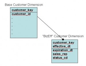
We will model this dimension with two tables as illustrated in Figure 1.  The dim_customer dimension table contains 47 columns–the customer key and all the other columns except the effective-dated columns.  The dim_customer_eff table contains 7 columns–the customer key, the effective date, the expiration date, the current row indicator, and the 3 effective-dated customer attributes. 

Figure 1: BizEff Dimension

The natural key of the base customer table is the Customer ID.  The natural key of the BizEff table is the customer ID and the effective date.  In both tables, the customer_id is replaced with an integer surrogate key.  The date key could also be replaced with a surrogate integer key.  Review Ralph Kimball’s definitive article on the rationale for surrogate keys.

The versioned BizEff rows represent contiguous and non-overlapping effectivity periods defined by the business effective and expiration dates. The effective date is provided the source system as entered by users.  The ELT application must derive the expiration dates for distinct sets of the effective-dated columns. The expiration date is 1 less than the effective date of the the next version.  The current version has a high value expiration date (e.g. 9999-12-31) as well as a TRUE value for the current row indicator. A change to any effective-dated column will trigger a new row in the BizEff table.  Note that if a particular column value does not change, that value is rolled forward to the next effective-dated row. 

If the number of effective-dated trigger columns is large relatively to the total number of columns in the dimension, or if the base dimension is relatively small, then there is not much advantage in splitting the base and effective-dated columns into separate tables.  Using a single BizEff dimension table will save a join when constructing the BizEff views.  There is no fixed rule about when to split a BizEff dimension into two tables.  You need to evaluate the capacity and performance implications for your particular situation.

BizEff Queries 

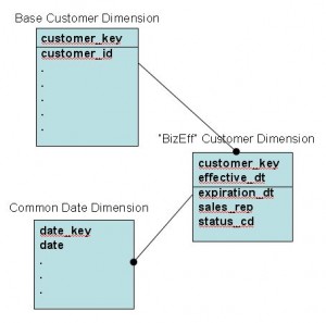
Now that we have a properly formed BizEff dimension, how do we query against it?  The trick is creating a BizEff view that conceals complexity from the client tool.  In the case of the 2-table BizEff customer dimension, the view joins three tables–the base customer dimension, the BizEff table and the date dimension (Figure 2).  The BizEff view returns a row for every date for which a distinct set of customer attributes is effective.  If the customer status for Suzanne Jones is Prospect from January 10 to February 12, the BizEff table would contain one row for that effective period and BizEff view would return 33 rows. 

Figure 2: BizEff AsOf View

The beauty of the BizEff view is that it can support both “AsOf” and “AsWas” queries.

  • AsOf queries group data according to the dimensional context in effect “as of” a user-supplied date.  The default AsOf date is normally the current date.
  • AsWas queries group data according to the dimensional context in effect at the time the fact transaction occured. 

BizEff queries are useful for companies that rely on the EDW for operational reporting.  This is particularly true for business processes that have inherent delays in processing demension updates.

Best of Both Worlds — BizEff2

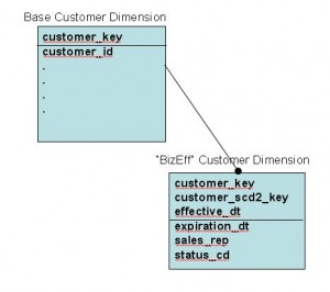
Just when you think you have satisfied the business users with an elegant BizEff solution, out comes a new requirement that sends you back to the drawing boards.  The accountants want to report how the transactions were originally recorded based on the incorrect dimension values–thank you very much Mssrs. Sarbanes and Oxley!  This requirement is met by including the standard Type2 SCD version key in the BizEff dimension table and in the fact table (Figure 3).  The originally recorded “as was” situation can be be recreated by joining the dimension table to the fact table using the the Type2 version key.  

Figure 3: BizEff2 Dimension
Note that with a BizEff2 dimension, it is necessary to preserve the original relationship of the scd2 key to the fact table.  This means that you could have multiple scd2 rows for the same BizEff effective date, or multiple effective dates for the same scd2 key.  This is more a more complex scenario but may be warranted in situations requiring maximum traceablity.
 

Performance Considerations

The performance implication of BizEff must be considered separately for ETL (back-room) and query (front-room) processing.  Traditionally, the brute force way to ETL late arriving dimension changes is to update the dimension keys for all affected fact transactions.  This approach approach works fine in data marts with relative small fact tables, but is not very scalable for rapidly growing fact tables with hundreds of millions of rows.  The BizEff approach is more efficient for ETL because it operates only on the smaller dimension tables.  Even very large versioned dimension tables are small in comparison to transaction grain fact tables.  

In general, BizEff queries perform somewhat slower than the standard Type2 queries because the the query uses expression joins to identify the correct dimension row.   Expression joins using “less than” or “greater than” operands are slower than the equi-joins used for standard Type2 queries.  The performance hit for AsOf queries is relatively light because the join of the static AsOf date is performed only once at the dimension level.  AsWas BizEff queries will perform somewhat slower than AsOf queries because the expression join must be applied to every fact row. 

With the performance of today’s MPP data warehouses, BizEff queries are a viable alternative to the brute force fact update approach.  Early performance testing will confirm the viability of BizEff for your particular situation.

*****

So the next time your users cry out for effective dated reporting, just tell them to them to go BizEff!

The EDW Moment

There comes a moment in the EDW life cycle when the light-bulb flashes on in someones mind.  Initially, this occurs with a select cadre of early adopters that “get it”.  Over time, and especially after the initial subject areas are successfully deployed, the lights flash with greater frequency. Eventually, the way forward is illuminated in every nook and cranny of the organization.  What makes the light flash is a very personal thing.  To the EDW practitioner, witnessing an “EDW Moment” is rewarding.  For me, they are what makes it all worth while.

In this post, I relate a few EDW Moments from my personal experience (names changed to protect the innocent), and invite you to share yours.  Such anecdotal successes are important to building support for an EDW initiative.  We need to understand the precipitating factors, formalize them in the EDW business case and ongoing management process.

The Go Get Bill! Moment

Certain types of memories make a lasting impression where you can remember visual details of the scene.  This happened to me at a client meeting in Florida where we were presenting a data warehouse prototype.  We had spent several days mapping out a dimensional model and loading the sales fact test data and a few dimension tables.  My colleague and I were executing queries against the prototype EDW in response to questions from the gathered managers and business analysts.  One manager commented:  “You know, one query we just cannot do today is the lifetime productivity of a sales rep.  At most, we can compute productivity based on prior year activity, and that takes all weekend to run.”

Well, let’s see…. SELECT sales_rep, region, SUM(act_rev) …… GROUP BY …. (2 minutes later) …. How’s that?

After a few seconds of stunned silence Suzanne, the IT director exclaimed, Go Get Bill!  Bill is the VP Sales Director down the hall. Bill came into the room and examined the query projected on the wall as Suzanne explained what had just happened.  I will never forget the look on Bill’s face.  It was literally jaw-dropping.  In an instant we had a room full of converts that “got it”.

The Drill-To Moment

Report drilling (clicking from summary to detail) is so fundamental to BI analysis that we sometimes take it for granted.  And yet, effective drilling is one of the most appreciated of BI features.  This point came home to me during the development of a maintenance reporting application for an electric utility.  We had spend several weeks gathering requirements and building up the maintenance subject area in the EDW.  Our business sponsor was a grumbly sort of hands-on manager, Ron, who got things done using static reports.  His main concern was getting more detail more quickly into his reports.  We explained the concept drilling into summary or exception reports, but it wasn’t quite registering.

Once the prototype was up and running, we gave a workshop for the section leads.  Things were going OK, but not great.  Then the drill-to moment happened.  Ron ask about some additional detail.  I clicked on a crew which had a  below standard schedule variance, bringing up the work orders for that period.  A number of the work orders showed a HOLD status due to materials unavailability.  Ron was visibly impressed.  I then showed him how we could further drill to see the personnel assigned for projects with productivity rates above/or below a threshold.  At that moment, Ron began the transition from BI skeptic to champion.

The Common Dimension Moment

Common dimensions evoke the whole range of emotions–from hope to frustration to elation.  They are challenging to introduce because of the perception that it is easier, financially and politically, to scope a solution around local requirements.  There is an element of truth to that perception, but it can be managed through an incremental approach to common dimension development.  Common dimension moments occur when when one or more common dimensions are already in production, or well along the development cycle.

Here’s the scene.  Business analysts and sponsors are laying out the requirements for a new EDW-based application.  You point out several areas that could be satisfied by common dimensions.  Nine times out of ten, this is welcomed news.  Not only does it reduce the project work scope, but sponsors recognize the value of tapping into a broader set of enterprise data.  It makes their job easier to sell the project to the funding powers at be.  I won’t say that there are high-fives all around, but common dimension moments are uplifting for all concerned.  Cultivating a climate for Common Dimension Moments, however, takes political will at the enterprise level.  Every EDW project must contribute in some measure to the advancement of common dimensions.  Your job, as EDW architect/evangelist, is promote the ROI of the common dimension strategy.

Your Mission

EDW moments are hugely important to a successful EDW initiative.  As EDW architect, your job is to create situations for EDW moments to happen, lock-in and follow-up aggressively when they do happen, and ceremonialize EDW moments to create a climate for change.  Think like a farmer—plant seeds with expectations that they will grow and bear fruit.  Then cultivate and water the emerging plants so they do.  Here is a short list of ideas.

  • Design prototypes to create EDW moments.
  • Do your homework.  Determine hot buttons in advance of key meetings and translate them into EDW scenarios.
  • Listen well.  EDW moments can be subtle and easily missed when you are doing all the talking.
  • Pursue mini-campaigns to solidify the EDW moment effects.
  • Build a story line that weaves together EDW moments to present a broader picture of the EDW impact.
  • Keep a notebook of EDW moments.  Take names, and track the progress of your follow-up campaign.
  • Make sure that the delivered EDW solution does, in fact, ring true to the EDW moments.  Calculate the risk of disappointment where it does not, and set expectations accordingly.

*****